Gradient Domain Fushion

Overview
This project explores gradient-domain processing, a versatile and impactful technique in image processing with applications in blending, tone mapping, and non-photorealistic rendering (NPR). The core of this project focuses on implementing Poisson blending, a method for seamlessly integrating an object or texture from a source image into a target image.
Part 1: Toy Problem
First, let's begin with a simple toy example. In this example, I'll calculate the \(x\) and \(y\) gradients of an image \(s\) and then reconstruct an image \(v\) using these gradients along with the intensity of a single pixel as a reference.
Let \(s(x,y)\) represent the intensity of the source image at \((x, y)\) and \(v(x, y)\) represent the values of the reconstructed image to be solved. For each pixel, we aim to achieve the following objectives:
-
Minimize \( \big(v(x+1, y) - v(x, y) - \big(s(x+1, y) - s(x, y)\big)\big)^2 \) \( \Rightarrow \) the \(x\)-gradients of \(v\) should closely match the \(x\)-gradients of \(s\).
-
Minimize \( \big(v(x, y+1) - v(x, y) - \big(s(x, y+1) - s(x, y)\big)\big)^2 \) \(\Rightarrow\) the \(y\)-gradients of \(v\) should closely match the \(y\)-gradients of \(s\).
-
Minimize \( \big(v(1,1) - s(1,1)\big)^2 \) \(\Rightarrow\) the top left corners of two images should be the same color.

Part 2: Possion Blending
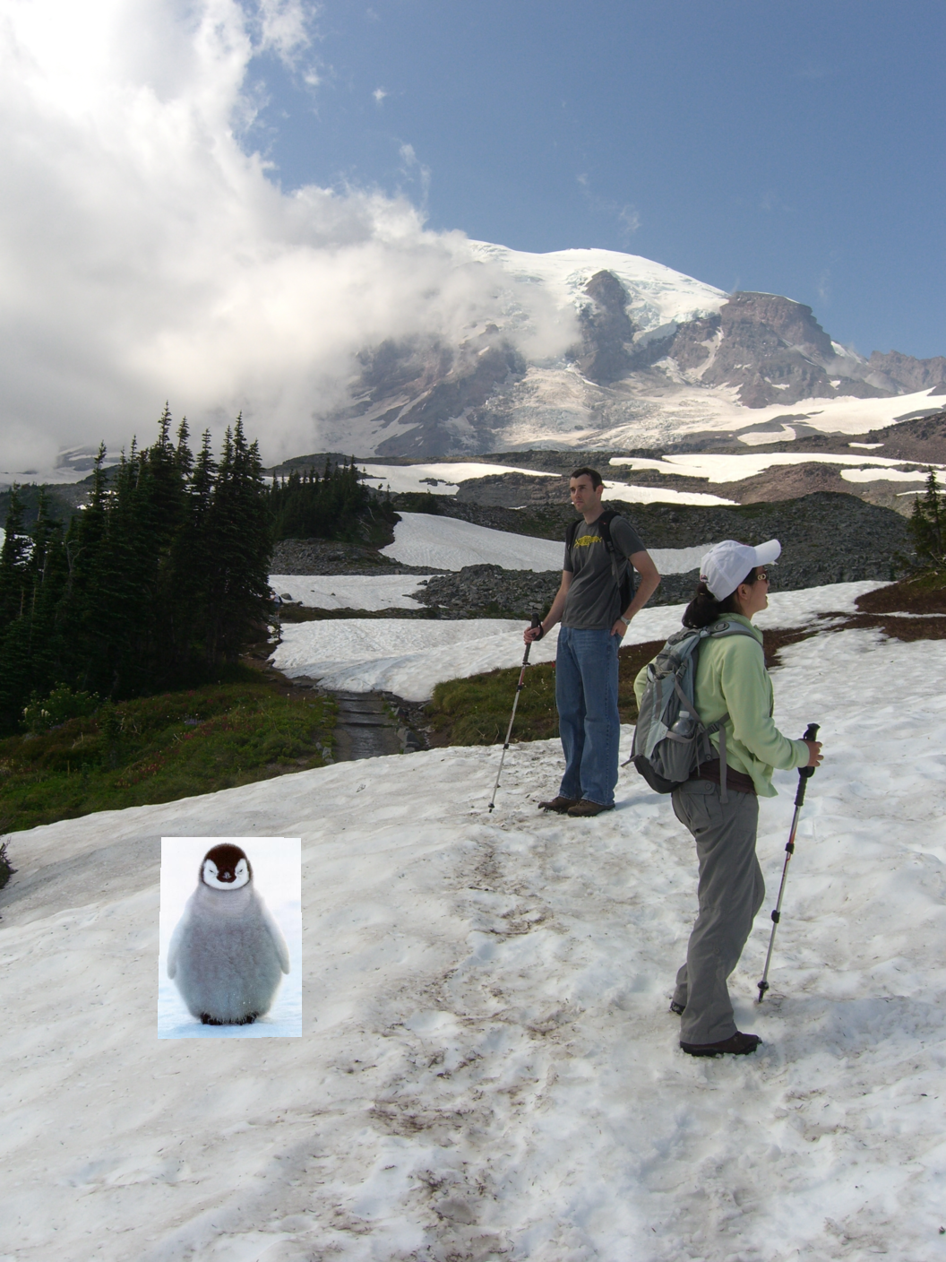
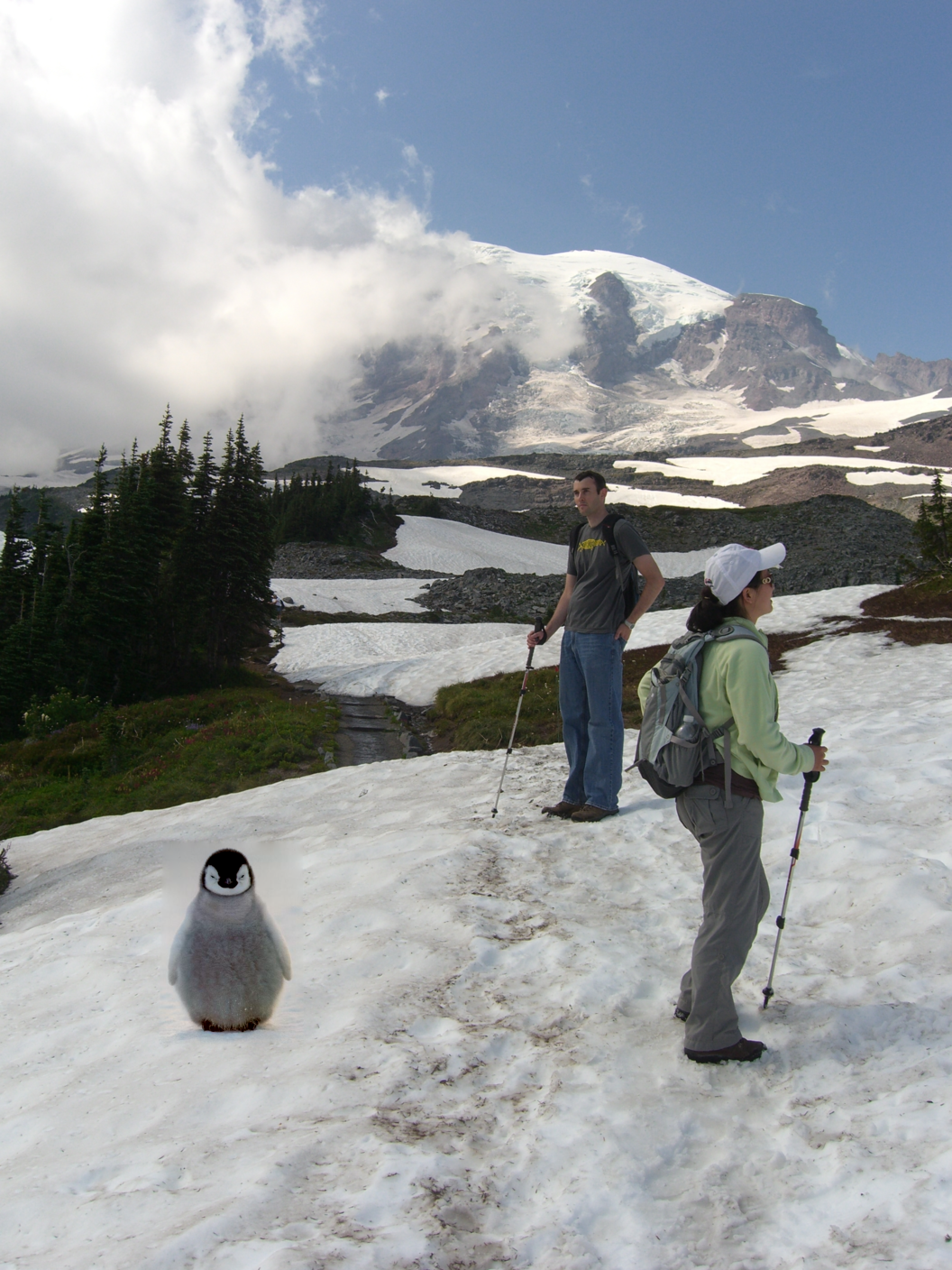
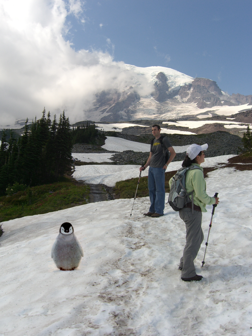
We will now explore an application of gradient-domain processing called Poisson blending. The goal is to seamlessly integrate an object or texture from a source image into a target image. Unlike our previous approach, we will focus on the gradients of the images. The challenge is to find the pixel values for the target region that best preserve the gradient of the source image, while keeping the background pixels unchanged. This problem can be formulated as a least squares optimization.
Given the pixel intensities of the source image \(s\) and the target image \(t\), we aim to solve for the new intensity values \(v\) within the source region \(S\), which is defined by a mask. The objective is: \[ v = \underset{v}{\arg\min} \sum_{i \in S, j \in N_i \cap S} \left( (v_i - v_j) - (s_i - s_j) \right)^2 + \sum_{i \in S, j \in N_i \cap \neg S} \left( (v_i - t_j) - (s_i - s_j) \right)^2 \] Here, \(i\) represents a pixel in the source region \(S\), and \(j\) is one of the 4 neighboring pixels of \(i\) (left, right, up, or down). The first term ensures that the gradients inside the source region \(S\) are as close as possible to the gradients of the source image we are inserting. The least squares solver smooths any sharp edges at the boundary of the source region by spreading the gradient mismatch over the interior of \(S\). The second term ensures that the boundary of \(S\) is correctly blended with the target image, directly taking the intensity values from the target.
Here is an example:
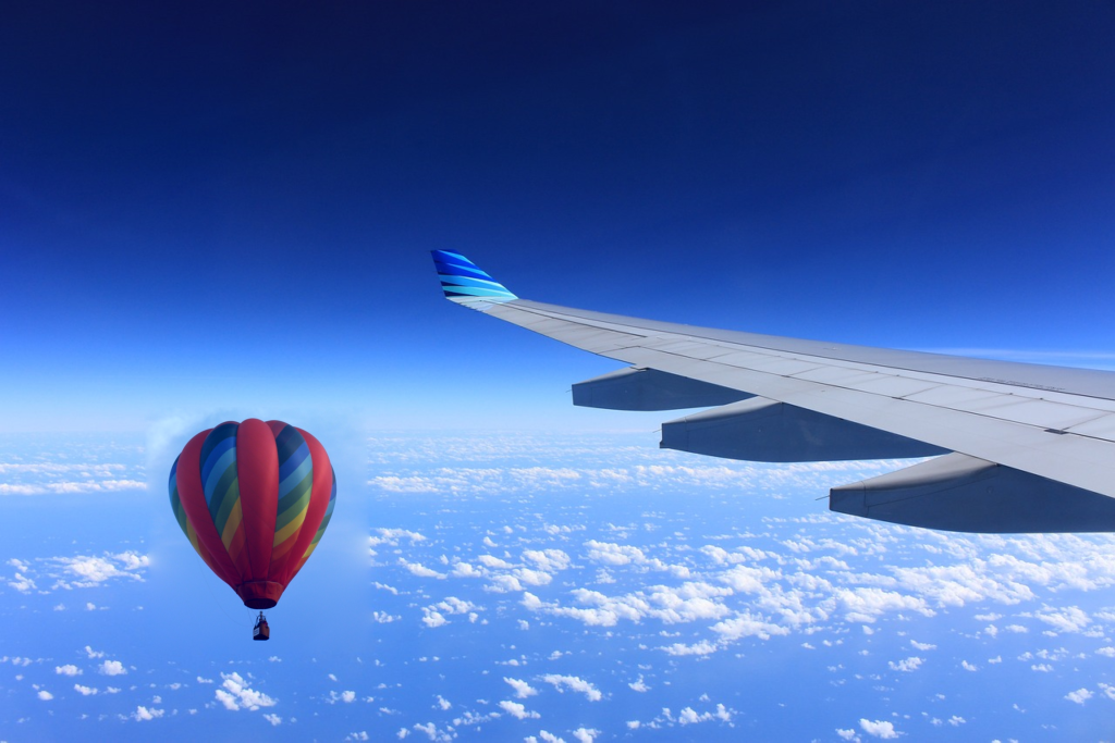
A few more decent results are shown below:
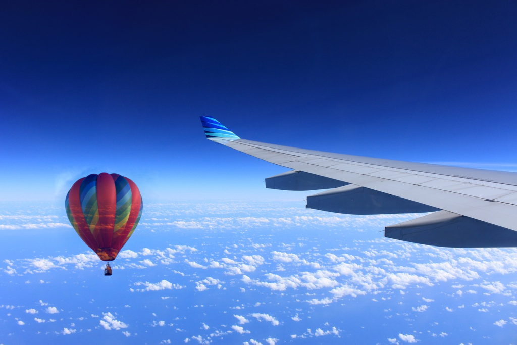
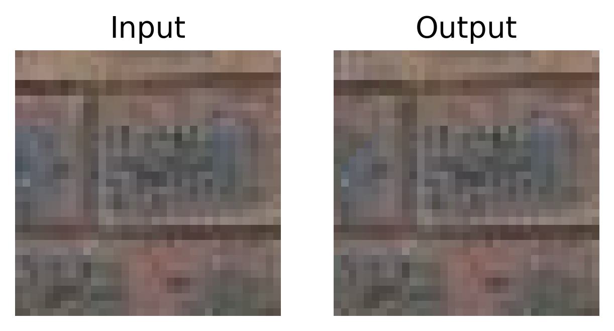
We now show a failure case:
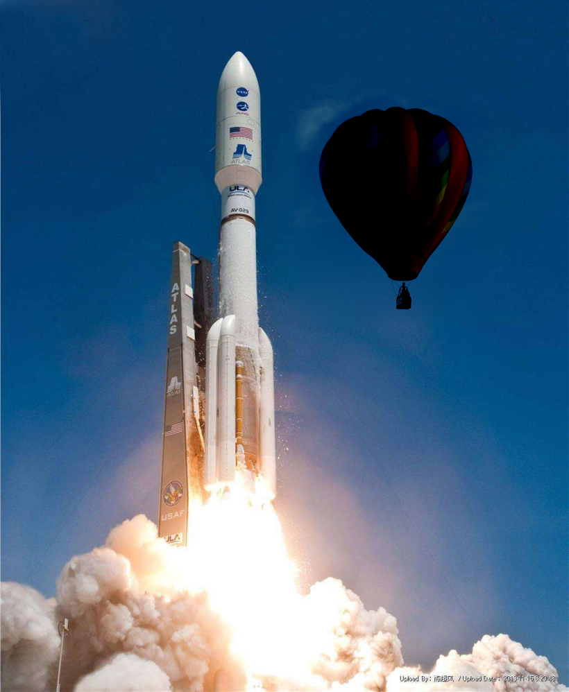
Although the blending around the source image was successful, the original color of the source image was not preserved. This issue is likely due to the significant color difference between the source image and the target image. As a result, the colors were drastically altered, with the colorful fire balloon attempting to match the dark blue of the sky.
Bells & Whistles
Mixed Gradients
Follow the same steps as Poisson blending, but use the gradient in source or target with the larger magnitude as the guide, rather than the source gradient: \[ v = \underset{v}{\arg\min} \sum_{i \in S, j \in N_i \cap S} \left( (v_i - v_j) - d_{ij} \right)^2 + \sum_{i \in S, j \in N_i \cap \neg S} \left( (v_i - t_j) - d_{ij} \right)^2 \] Here \(d_{ij}\) is the value of the gradient from the source or the target image with larger magnitude.
In the example below, you could notice that mix gradients blending performs better as it blend the border of the source image with the target image, which makes it looks more natural.
In addition, the source image becomes semi-transparent after mix gradients blending, so mix gradients blending might perform worse in some case, such as the target image is complex:
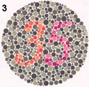
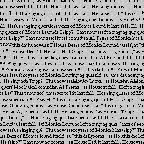
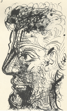
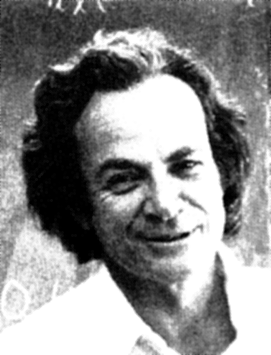
Color2Gray
When converting a color image to grayscale, such as when printing to a laser printer, important contrast details can be lost, making the image harder to interpret.
To preserve the details, I utilized gradient-domain processing to create a grayscale image that retains both the intensity of the rgb2gray output and the contrast of the original RGB image. This approach is conceptually similar to tone-mapping, often used in converting HDR images for RGB displays.
By converting the image to HSV space, I analyzed the gradients in each channel, and then formulated the task as a mixed gradients problem. This method allowed me to preserve both the grayscale intensity and the contrast of the original image. The final grayscale image I produced was shown to maintain the contrast information while keeping the numbers easily readable.
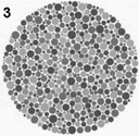
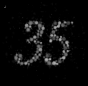
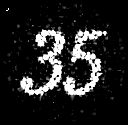
In addition, I noticed that I could make the result even clearer if I scale the grayscale intensity by some large ratio, e.g. I use 5.0 here.
Cool Stuff I Learnt
This project has been a lot of fun, especially the color2gray part! I really enjoyed the visualization process. Most importantly, it has deepened my understanding of blending and gradient-domain processing. I now have a better grasp of the relationships between different color spaces.
Image Quilting
Overview
In this project, I implement an image quilting algorithm for texture synthesis and transfer, as presented in the 2001 SIGGRAPH paper by Efros and Freeman.
Texture Quilting
The goal of texture quilting is to fill a larger image using the texture from a small sample image in a way that appears natural to the human eye. Below, the results are shown along with explanations of each method.
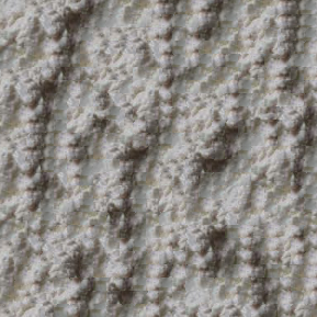
Randomly Sampled Texture
This technique fills the target image grid-by-grid, but the grids are significantly smaller than the size of the texture image. Each grid is randomly filled with a patch that is uniformly sampled from the texture image. We randomly sample square patches of size patch_size from a sample in order to create an output image of size out_size. Start from the upper-left corner, and tile samples until the image are full.
patch_size = 55, out_size = 331Ovrelapping Patches
You could observe that using random patches alone does not address the discontinuities along the borders of each grid from the last part. To minimize these discontinuities, a better approach is to fill each grid with patches that are similar to the neighboring grids already filled along the borders. We could realize this using overlapping patches. When a grid is being filled, the pixels in the texture image just outside the candidate patches are compared with those in the neighboring filled grids using the sum of squared differences (SSD). Patches with lower error are preferred for filling, ensuring a smoother transition between the grids.
patch_size = 35, overlap = 9, tol = 1Seam Finding
However, using patches with similar borders still leaves some noticeable discontinuities. To improve the use of overlapping patches, patches are pasted into the target image with their borders masked in a way that ensures smooth transitions from the already filled grids to the new patch. That is the seam finding technique.
patch_size = 35, overlap = 9, tol = 1The technique of seam finding is that, there could be a way to cut and stitch two overlapping patches such that the transition between the two patches is seamless, even though they may not perfectly align. One approach to find this cut is to identify a path in the overlapping region where pixel value differences are minimal. If the pixel value differences along the best such path are small, it suggests that the two patches are aligned along that path. Assuming the textures are repetitive, the texture content on either side of the path should also repeat, making the transition less noticeable if the patches are stitched along this path.
Here is the illustration of finding such path:
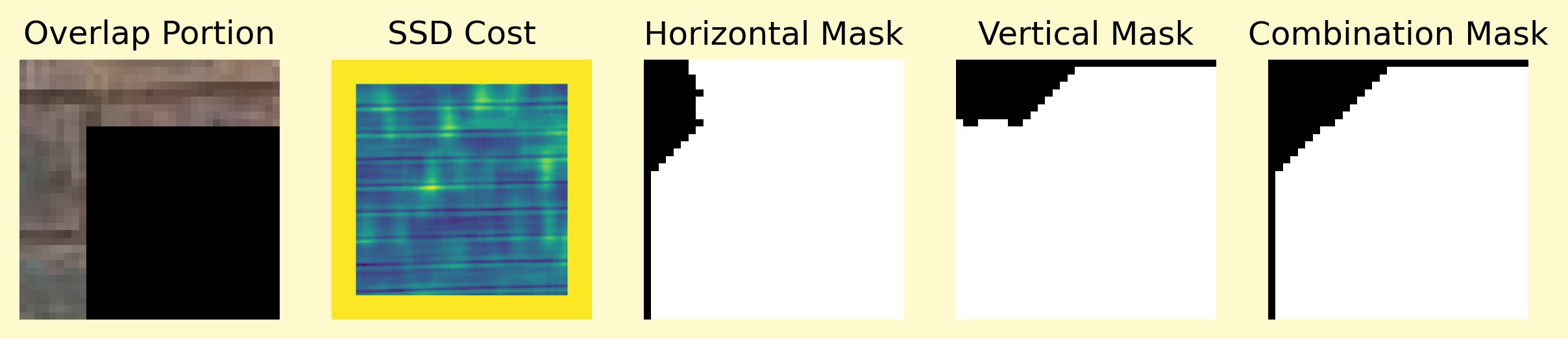
After applying the mask, we got the seamless patch:
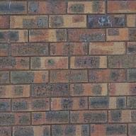
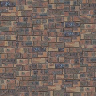
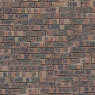
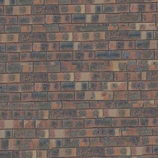
Below are four additional texture quilting results where the overlapping with boundary cut technique is applied to create textures with double the size. The source texture images are displayed next to their corresponding quilted images.

patch_size = 15, overlap = 3, tol = 1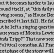
patch_size = 25, overlap = 5, tol = 1Texture Transfer
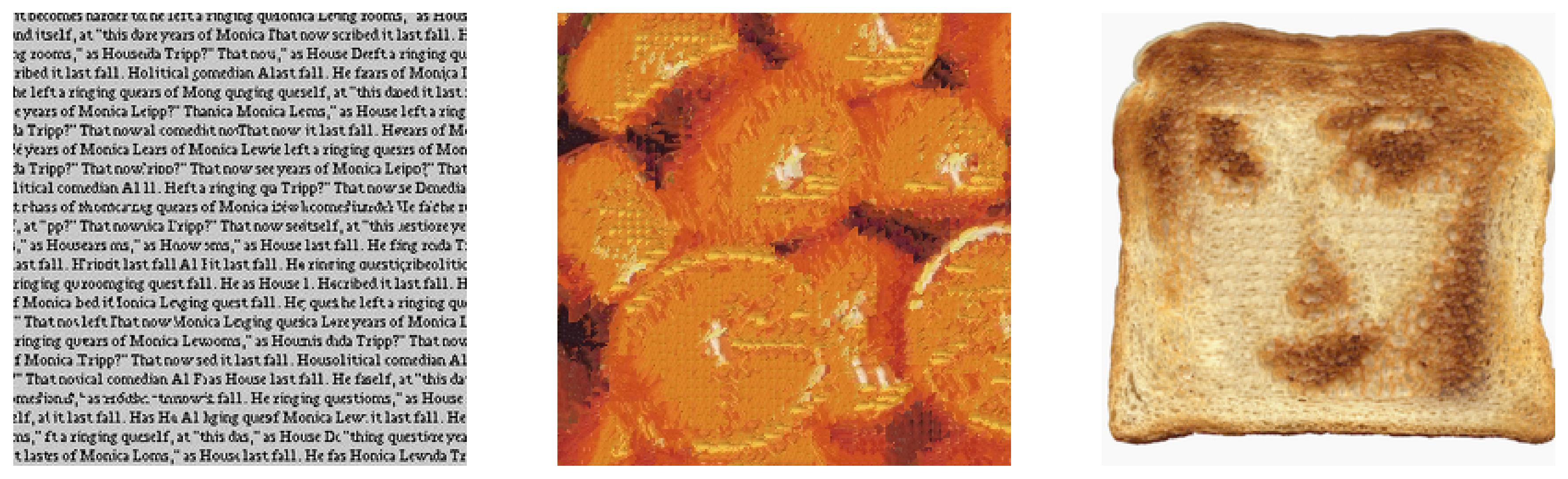
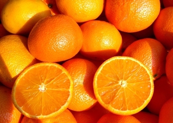
The texture quilting technique of overlapping with boundary cut can be extended to perform texture transfer, which aims to reconstruct a target image by using textures from the texture image to create a version of the target image embedded with the texture.
The procedure used for texture transfer is similar to the seam finding technique used for texture quilting. The key difference is that the cost image is calculated as the weighted average of the SSD of the sample image and the SSD of the guidance image. Here when the ratio of sample increases, the result would look more likely to the sample texture, while decreasing the ratio would result in an output like the guidance image.
patch_size = 27, overlap = 5, tol = 1, alpha = 0.9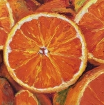
patch_size = 13, overlap = 8, tol = 1, alpha = 0.3Bells & Whistles
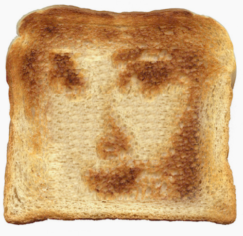
Image Blending
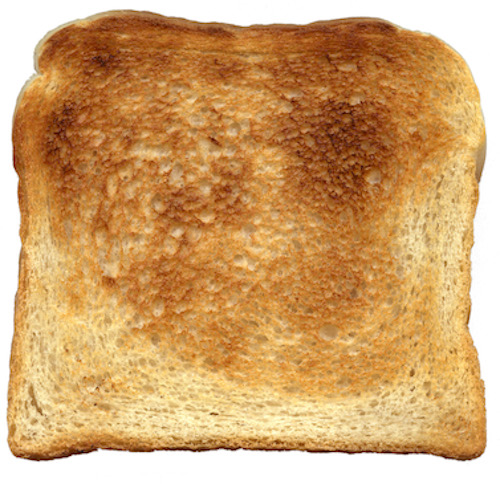
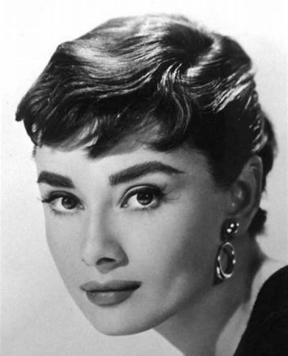
First, I transfer the face into toast texture.
patch_size = 25, overlap = 10, tol = 1, alpha = 0.7Then I cut the output and resize them into the size of toast to create the appropriate mask.
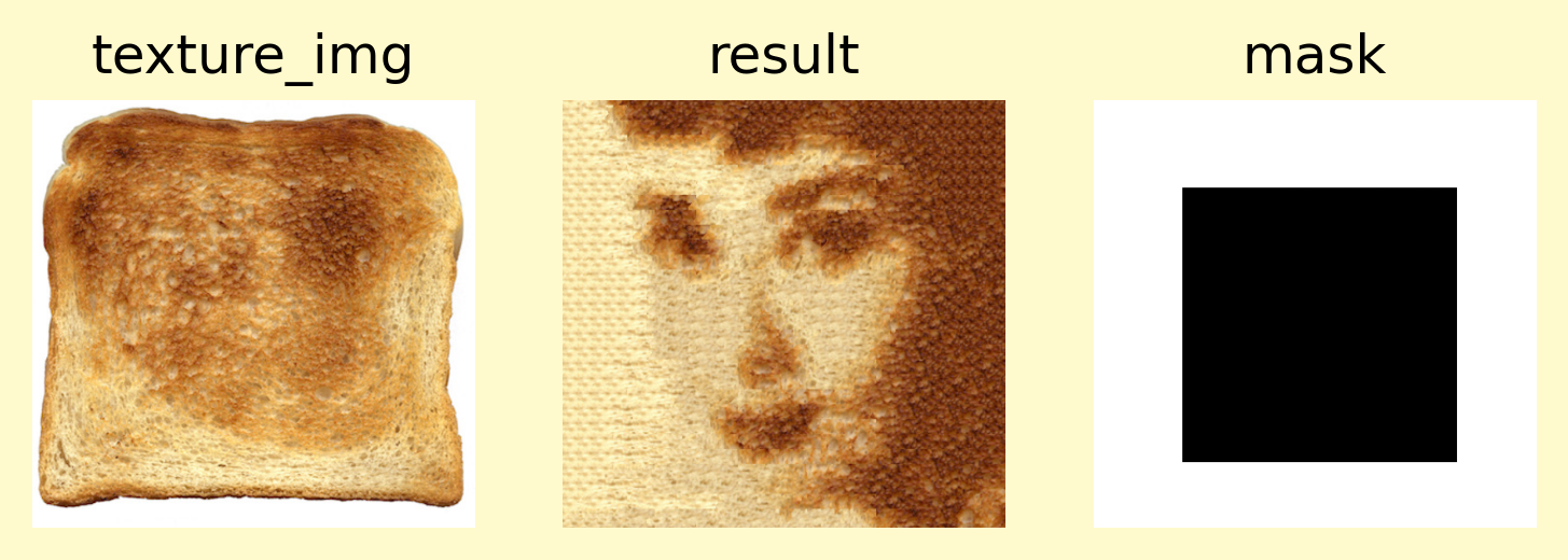
Finally I use the Laplacian stacks to create the face-in-toast image.